
|
|
Sound is a variation of atmospheric pressure that naturally dissipates at a fixed rate outward from its source. We perceive a specific pitch when the sound pressure varies at a constant rate, alternating positively and negatively from normal atmospheric pressure. The range of pressure oscillations that we can hear extend from the lower frequencies that we actually feel, to about 15KHz. Depending somewhat on relative humidity, the higher frequencies are diminished as they propagate through air, due to losses that affect the lower frequencies to a lesser extent. Microphones can pick up this pressure variation and convert it to an analog signal, a voltage that varies continuously with time, accurately representing sound pressure variation. Analog circuitry can be used to process this signal, using amplifiers, resistors and capacitors, but analog components are never precise, the circuits are difficult to build, and the components may change slightly due component to aging over time. Digital techniques are now available to quantify the analog signals in both amplitude and time to form a sequence of numbers that represent the analog signal so that mathematic techniques can be used to process the signal. Although this quantization does represent a potential defect in the process, once the sound is converted into numbers, the processing step is fixed and invariable; within the limits of the signal quantization, the processing is mathematically perfect. In order to convert a continuously varying analog signal into a regularly spaced series of numbers, the signal must be sampled at a constant rate. Each sample represents the signal's value at a precise instant in time. Each sampled value can then be converted into a binary number that numerically defines the sample's value. This analog-to-digital conversion (ADC) produces a continuous stream of numbers that can then be processed with digital techniques. After processing, the resulting samples are sent to a digital-to-analog converter (DAC) so that the reconstructed analog signal can be sent to amplifiers and speakers or headphones. The rate at which the analog signal is sampled will determine the highest frequency that can be accurately converted, and the size of the digital numbering system used will determine the accuracy of each sample's conversion. A signal can be sampled like this:
This is a sine wave, a pure tone with no harmonics, that is sampled at a regular rate. Although the entire waveform is not represented in the finished samples, the exact same waveform can be reconstructed from such infrequent sampling, provided the process is continuous and the samples are ultimately passed through an appropriate filter in the DAC. If the signal frequency is too high, or the sample rate is too low, then aliasing will occur:
The original signal is shown as a black line, and is sampled at too low a frequency, less than 2 samples per cycle. Upon reconstruction in the DAC, the purple waveform results; a signal of lower frequency than the original. This lower frequency is called an alias ('by another name') of the original input, and happens whenever the sampling frequency is less than twice the frequency being sampled. Since alias signals are not at all related musically to the original pitch, aliased signals sound extremely unnatural and must be avoided through proper anti-alias filtering prior to the sampling process. **** Note: To properly sample the audio band that humans can perceive, without objectionable aliasing, an appropriate maximum sample rate is perhaps 40KHz. The choice of the 44.1KHz sample rate for the Compact Disc was a good one, as it allowed the preservation of 20KHz as a maximum frequency limit, a band 'edge' that has been long accepted as the upper limit of the human hearing system. In fact, few people can hear beyond 16KHz. In certain circles, it is politically incorrect today to infer that higher sample rates have no benefit, for there are many audio engineers and well respected people in the audio community that insist 96KHz or even 192KHz sample rates demonstrate improved subjective audio quality. In fact, due to continuing technological developments, audio quality has improved from the days of hissing tape and high distortion analog electronics to the point where such 'experts' now feel they have little to contribute but these unfounded opinions. Nothing within sampling theory or the mathematics of signal processing, or hearing measurements on individuals lend truth to these claims, and they are therefore in the realm of belief. Thus, the Church of Modern Audio is born. Sadly, if your customers belong to the Church, then you will be compelled to belong too, for this belief system does not tolerate heretics. It is interesting to note that many producers today will master their work at 96KHz, with 24 bit resolution, and then distribute their work on a low rate MP3 format. Go figure. No two loudspeakers sound exactly the same. A-B listening tests can repeatedly reveal one choice to sound 'better' than another by simply having a fraction of a dB more loudness. The days of low quality audio are over, and perhaps, in the interest of producing better music, the emphasis should be on songs, talent, arrangement and novel effects, not imperceptible 'improvements' upon something that is, for all practical purposes, perfect. It is interesting to note that the best selling music of all time was produced on analog tape, in a completely analog environment! This is not to say that the lower quality systems of yesterday were somehow necessary to good music production, it is to say that talent and engineering artistry may be more important than inaudible technical details. The economic reality of consumer electronics marketing however, demands 'newness'. In the absence of real value added to the last model, at least 'perceived' value will do. This in fact, is the origin of higher than necessary sample rate systems, despite the built-in inefficiencies of storing and processing twice or even 4 times the required data. When the marketing hype required to explain this new 'advantage' is produced, the result verges on dishonesty. You must decide for yourself what is most important when you design and market your product; my hope is that you can bring real value to your work. ****
Analog to digital converters produce binary numbers at the sample rate, each number representing the analog input signal value at a sampled moment in time. The width of these binary numbers determine the possible resolution of the conversion. Binary numbers can be of any conceivable number of bits wide. A 16 bit number (CD quality) is capable of resolving an amplitude detail that is 1/65536 of the maximum signal amplitude, causing an error in the conversion that is about 96dB down from a maximum signal. When converting low level signals, this quantization noise may become objectionable. During careful listening to selected signals in a quiet environment, quantization noise that is roughly 70dB below a signal can just become noticeable, so CDs are usually mixed toward the 'hotter' side, some even clipping from time to time. The use of a wider bitwidth, such as 20 or 24 bits is helpful in reducing the effects of amplitude quantization, but analog noise will invariably obscure the ultimate dynamic range of an ADC or DAC. The maximum dynamic range of the human hearing system is perhaps 105dB, from the loudest sounds that are uncomfortable to continually endure to the faintest noise when all is quiet. In practical environments, with air conditioning systems, computer fans and natural sounds around us, a practical dynamic range may be 75 to 85 dB. Most powered speaker systems, even those of studio monitor quality, have a maximum dynamic range of perhaps 95dB from the peak acoustic signal at clipping to the residual noise from the tweeter.
Once in the digital 'domain', binary samples can be manipulated mathematically. Samples can be stored in memory and read out at a later time (delayed), multiplied by some constant number (providing gain or loss), added together (mixing), or combinations of these operations, leading to filters (such as tone controls) and effects. The audio signal processor will repeatedly execute the same algorithm on each incoming sample, producing one sample out for every sample in. The algorithm is a list of mathematical operations to produce the desired result, and one or more algorithms will constitute a program that is written by the programmer and downloaded to the processor where the processor will continuously execute the algorithms on the sample stream. Signal processors require the ability to store samples and add (or subtract) and multiply sample values by constants or other sample values. Each processor has a fixed architecture, an organization of processing elements that are capable of these functions. Manufacturers produce DSP processors with different architectures and therefore different lists of possible instructions that suit the architecture's capabilities. Programs are written in the human-readable language of the specific processor, using unique commands mnemonically abbreviated, such as MOV (move), ADDC (add with carry), and so forth. The instruction informs the processor what to do, and is usually followed by arguments that instruct the processor as to what memory elements or constants to use in the operation. Usually, each line of the written program is an individual instruction command. The written program is then assembled into control information, a distillation of the written text, into a compact list of control words that the processor will store in its control store memory. During execution, the processor will fetch these control word instructions one at a time, and execute them in order. For the purpose of discussing DSP operations and planning algorithms, a schematic technique has been developed that will be used throughout this discussion. Arrows show the direction of signal flow; an arrow into a device will obviously be to an input. Device outputs do not require arrows. Circles with a + or x inside represent addition and multiplication respectively. Sometimes the coefficient used in a multiplication is inserted into the circle in place of the 'X'. Subtraction is performed by writing a - sign by the arrow of a signal as it enters an addition. Adders may have any number of inputs, but multipliers usually have only two input arguments. A box represents a single sample delay (one memory location) if empty, but may represent a longer delay (more memory elements), indicated by a number within the box. A single memory element is often called a register. Boxes may also represent other functions, but will be clearly indicated with text inside the box.
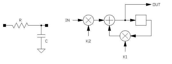
As an example of a short and simple algorithm would be that of a low pass filter:
The coefficients K1 and K2 can be calculated to provide a required -3dB response, but we can actually examine the behavior of the algorithm to determine these values, at least roughly. We begin by realizing that K2 is an input gain control only, and set it to 1.0 for our experiments, to see how the rest of the algorithm behaves. Let's set K1 to 0.5 to conduct our experiment. We will begin by imagining the input has always been zero, and that the value in the register (empty box, only one memory location) is also zero. We will then cause the input to be a +1.0 value, and watch what happens on each algorithm iteration. When evaluating algorithms, it is important to establish an order of events. In this case, we will state our algorithm as:
If we track the value in the memory location, we find the following sequence: 0 * 0.5 + 1 = 1.0 From these few iterations we can see that the result is slowly approximating to 2.0. From this we can speculate (correctly) that the filter has a DC gain of 2.0, and to make it have unity gain, a K2 value of 0.5 would be required. Further experiments reveal that for a unity gain filter of this structure, K1 and K2 will both be positive, and their sum will equal 1. Therefore, as the K1 value is increased, K2 will become smaller, indicating that the filter has a higher intrinsic gain as K1 approaches 1. At a K1 value of 1.0, the gain of the filter block would be infinite, and K2 would be forced to zero to compensate; this is no longer a useful filter. If we plot the step response of an analog RC filter:
We know the time constant is equal to R*C, and can calculate the -3dB frequency of a filter with 1/(2*π*R*C). We can also see that if we draw a straight line, as parallel as possible to the starting portion of the RC time constant waveform, the line will intersect the final approximated value at the TC point in time. Likewise, if we know the rate at which our digital low pass filter is beginning it's asymptotic approach to the final output value, we can obtain an equivalent RC time constant. From this we can determine the -3dB frequency. Techniques like this, following the process through experimentally, will give you a deeper appreciation for the mechanisms at work in DSP algorithms, and will be revisited later in these pages. By the way, the proper formula for a simple, single pole filter such as this is: K1=e-(2*pi*F*t) Filters will be discussed in greater detail here.
|