
|
|
Programming the FV-1 :: a quick setup tour
FV-1 programs should begin with memory declarations and equates for variables. This is so that they may be accessed easily, as programs can be written so that constants and delay values can be referred to many times within the program; declaring a familiar name, like RevTime. These labels may be used many places within a program, and if entered once at the top, their influence through the entire program my be had by changing only a single value. Further, the SpinAsm assembler is a two-pass assembler, so equates and memory declarations may be made anywhere within the program, but placing them all at the top allows the programmer the advantage of seeing that there are no unintended conflicts; the assembler will allow two labels to equate to the same register, which may not be the programmer's intention. The bulk of the code follows, and can be liberally commented. A semicolon stops the assembler from parsing further on a line, so semicolon-preceded comments can be inserted anywhere. Spaces between lines can be used without a semicolon if desired to make the code more readable. One-time setups, such as the loading of LFO information should be done before the LFO is referenced by code, and would most logically be the first instructions in the program, preferably following the list of memory declarations and equates. No end statement or other end-of-program identifier is required. All keywords, opcodes and label names are case insensitive.
To declare an area of delay memory for later use, the MEM statement is used. The format can be either:
When using the label in instructions, the label name points to the beginning of the delay, the label followed by a # (no whitespace between) refers to the end of the delay, and the delay name followed by the ^ symbol refers to the midpoint of the delay. Usually we would read from a delay endpoint and write to the delay beginning. Delay midpoints are useful when the delay is to be +/- swept by an LFO. The assembler will allocate memory for each declared label and delay length. Be aware, since the end of one delay must be at a different physical address from the start of the next declared delay, the number of delay memory locations used will be one greater than the declared delay for each delay declaration. Variables can be given names with the EQU statement, and as with the MEM statement, may either be the first or second entry on the declaration line. Labels may be equated with equations, numbers in decimal, binary (preceded by the % symbol) or hexadecimal (preceded with the $ symbol). Also, registers may be assigned to label names, so that they may be referred to in a program by a familiar and relevant name, and the inadvertent use of the same register in two different places can be avoided. Labels may be anything you like, but they must not have a numeric starting character, and may not be a reserved word.
While using the SKP command, the number of lines to skip can be entered directly, or alternatively, the skip may be to a point in the code that is uniquely labeled thusly: LOOP: The label may be any unused, unreserved label, followed by a colon, all by itself on a line. The assembler will calculate the number of instructions to skip, automatically.
The two audio inputs are ADCL and ADCR, while the outputs are DACL and DACR. these are read and written as registers, much as you would the register bank REG0 through REG31. DAC registers cannot be read from, nor can the ADC registers be written to. POT0 through POT2 are control values that will span 0 to 1.0, depending on the pot pin's input voltage. Between the ADC inputs and the DAC outputs, a program must be written that performs the desired function, possibly using the POT values in the process. The architecture of the FV-1 is centered around the accumulator, abbreviated for speaking terms as ACC. For an efficient signal flow through the processor, the signal will often be present in the accumulator when entering a code block, and the result of the process will be in ACC when the code executes. Work toward finding code sequences that permit this, as opposed to less efficient routines that must store ACC temporarily in a register. There are cases however, where this cannot be avoided. Many of the opcodes perform additions to ACC, so it is a good idea to always end a program with ACC=0. Since the last line of a program is often (but not necessarily) the writing of the accumulator to a DAC output, setting the coefficient during that operation to zero will leave ACC cleared, ready for the first instruction to be an addition to the cleared accumulator. This is a good coding habit to consider. The ability of the instruction set to clear (coef=0) or maintain (coef=1) the ACC value during register or delay memory writes is handy when writing signal processing code that flows nicely. Many frustrating coding errors are due to an unintended write coefficient value. Check this first when debugging your code!
Full programs that include the use of the potentiometer control inputs will have several sub-sections that set up and possibly scale, filter and offset the pot values so derived results may reside in a register for use within a program. The pot values range from 0 to 1, quantized at the 9 bit level (513 possible values), and have hysteresis applied, so that a small amount of noise on a pot input will not cause the jumping between two adjacent codes. The pots can be used directly to control parameters within your code, but you may wish to filter them first:
Notice, the last write used a coefficient of zero. If the sub process is not preceded by a write that cleared the accumulator, it will be carried into the calculation. Pots can be scaled with the coefficient that is used when they are read, and offsetted by a value using the SOF instruction. In the above filter, the register called pot0fil is being read, added to the pot input and written back to pot0fil, giving the structure a gain of 1-(1/0.99), or a gain of 100; the pot is read by a coefficient of 0.01 to compensate for this gain. The resulting pot value though, used as a coefficient for controlling something, will have relatively smooth transitions as the pot itself steps through its output codes. If the pot value is intended to control a parameter and the linear pot value is not as desirable as say, an 'A' taper potentiometer characteristic, consider scaling the pot with the following:
This will effective multiply the pot0 value by itself. The result will be a numerical output of 0.25 when the pot is centered. We have effectively squared the pot value. Using two such MULT operations will effectively deliver the cube of the pot input value, and so on. Pot values can be inverted and scaled too. Consider this code:
This will cause the accumulator result to be -0.2 when the pot is at zero, and +0.6 when the pot is producing a 1.0. Between these extremes, the ACC value will linearly track the pot input. Techniques like this can be used to scale pot values for preparation to drive EXP or log functions, or control compressors or LFOs.
The ADCs are equipped with a fixed high pass filters, rolling off the lower frequencies at a few Hz, to remove DC offsets; otherwise, slight DC offsets at the inputs could cause unpredictable behavior, especially with recursive DSP algorithms. The DACs however, have response down to DC, and can be used to test your algorithms, especially those that derive control signals from pot inputs. If you have problems getting a pot function to work the way you want, send the result to a DAC output, and watch the signal's behavior with an oscilloscope attached directly to the DAC pin. 0 will be shown as a mid-supply value, and positive and negative values can be displayed over the maximum of the processor's signal value range. This is a great technique for evaluating the rather complicated LOG and EXP functions. The DACL pin is at the top of the package, easy to clip onto, and is the preferred output for such testing.
You will notice that the read and write instructions are divided into those those deal with delay memory (RDA, WRA, WRAP) and those that deal with registers (RDAX, RDFX, WRAX, WRLX, WRHX, MULX). The two kinds of memory have different qualities and are used for different purposes. Registers are 24 bits wide, with the exception of the POT inputs, that offer 9 bits of resolution. Operations that require high precision should be done using these registers and their corresponding opcodes. On the other hand, delay memory is addressed differently, so that delays can be easily built, and the data storage technique is different, a floating point representation. This data storage scheme allows a 26 bit dynamic range, but a limited resolution, resulting in very low level distortion products. If the registers are used for delay, the addresses will need to be calculated in the algorithm, and if the delay memory is used for applications such as low frequency filters, some distortion will result. The opcode set has been optimized to execute subsets of code for various common audio tasks; the all-pass filter for example, is executed by only 2 operations, but must do this from delay memory with the RDA and WRAP operations. When used in a reverb, where perhaps a dozen all-pass filters may be required, this is very efficient. If however, you wish to impliment an all-pass filter with a delay of only 1 sample, the RDA/WRAP scheme could be used, but only if the coefficients in the all-pass are not too extreme. Coding low frequency all-pass filters will require a less efficient set of operations using registers for storage. On the other hand, low frequency filters benefit from the use of high precision memory, and can be efficiently calculated using registers and the RDFX, WRLX and WRHX commands. Single pole low-pass and high-pass filters can each be built as two instruction pairs on a register. Further, these filter structures accept ACC as the input and provide the output in ACC, ready for the next stage of processing.
Preparing pots to control processes The control inputs will deliver a 0 to 0.998 signal, quantified to 9 bits, with hysteresis added to ensure that vibration or supply variations do not cause the value to jump between adjacent codes. The pots can be used directly for many purposes, but their values can be modified to suit particular needs. 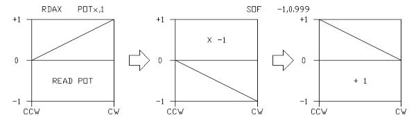
The above shows the preferred method of 'flipping' a pot function. Alternatively, if the accumulator is not cleared prior to the operation, the following would do the same, while clearing the accumulator in the process:
The first method is clearer, but the second can be used to solve the problem of a non-zeroed accumulator which may result at the end of a skip operation that is conditional on the accumulator status. In either case, the final value resides in the accumulator and can be written to memory or registers as desired. The accuracy of the finite math, and the 2's compliment numbering system cause slight inaccuracies, but the 'zero' value from the pot is guaranteed, and the slight error between the maximum positive constant in the SOF operation and a true 1.0 is usually negligible in effects design (0.00869dB). Although the assembler will not accept a full 1.0 value as a constant (although it will accept -1.0, which is a valid 2's comp number), I may refer to 'adding one' in casual process descriptions. The pot function can be 'shaped' by several means: 
This is simply a squaring process, multiplying the pot value by itself, to approximate a logarithmic, or audio, taper. After the first multiply, the midpoint of the pot travel has moved from 0.5 to 0.25, after the second multiply (cube) it becomes 0.125. Of course, if required, this result can be 'flipped', as above, or, the squaring (or cubing) process can be applied to a 'flipped' version. Since the numerical processor within the FV-1performs saturation limiting on all processed signals, the pot value can be clipped against the processor's limits:  Here, we've used the SOF -2,0, only because it's convenient to type, and because we needed to use it twice. We could have used two SOF 1.999,0 as well, and the signal would not have changed sign in the process. The final function could be used to crossfade between two signals at the onset of pot rotation, at the counterclockwise end. Signals are most easily cross faded by the following process:
The idea is that when xfade=0, only the A signal remains in the accumulator at the end of the cross fade process. If xfade=1, then the B signal will get through, and the A signal will subtracted from itself, and will therefore not contribute to the output. Xfade values between 0 and 1 will lead to a mixture of A and B. Consider the following: 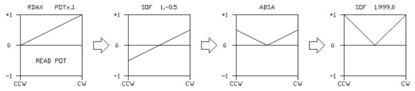 Using this visual approach to forming control functions, a single pot process can be quickly imagined to derive any desired final control value. To provide yet further flexibility, the LOG and EXP functions can invoked as well. The pot control values can be used directly, or tweaked in the above fashion to control many functions directly. Because the pot functions are quantized to 9 bits, in some cases the discrete jumps between output codes can be distracting; in such cases the control signal can be easily filtered to produce a smoother control output:
The value potfil can now be used as a 'smoothed' version of pot0.
The two RAMP generators and the two SIN/COS generators, collectively called the LFOs, are a powerful part of the FV-1's capability. However, their flexibility and range of usefulness causes a degree of complexity that cannot be considered lightly. You must thoroughly digest the information presented on these sub-functions before using them, as the simple copy and paste method of using example code may be frustrating at first. Both SIN/COS and RAMP generators have parameters of frequency and amplitude that must be established for them to behave as you would like, and the parameters are different for the two types. The SIN/COS LFOs have a frequency value that allows a 9 bit range of LFO rate, spanning from one cycle every 24 seconds to about 30Hz when clocked with a 32768 crystal. The LFO rate will be linearly related to clock frequency. The amplitude of the SIN/COS block will depend on the amplitude parameter, a 15 bit value. The SIN0 (for example) generator is initialized once, at the top of the program for continuous operation by writing:
The two lines of code will set the parameters for the SIN/COS0 only once, as after the program has executed over one sample period, the RUN flag will be set, and the WLDS instruction will be skipped over for all subsequent sample cycles. The value freq will be an integer between 1 and 511, the value amp will be a value from 1 to 32767. Both are linear controls. For the RAMP generators, the initializing opcode is WLDR, the LFO is selected with either RMP0 or RMP1, and the parameter for freq is 16 bits, a 2's comp value, set between $8000 (maximum negative) and $3fff (maximum positive). The amplitude is fixed at 4 possible values: 0 provides an output range of 512, 1 provides 1024, 2 provides 2048 and 3 provides 4096. These are output ranges that are expected to be added to a memory address when sweeping a delay automatically. The LFOs can be initialized once with a WLDS or WLDR command, protected by the SKP operation and left to run, or they can be modified 'on-the-fly' by writing to the registers LFO(X)_RATE and LFO(X)_RANGE, where (X) denotes the number of the LFO. The SIN/COS0 and SIN/COS1 are represented by the numbers 0 and 1 respectively, while RAMP0 and RAMP1 are represented by 3 and 4 respectively. When writing to these control registers within a program, it will be from a calculation the result of which resides in the accumulator. The upper bits of the accumulator are used for this purpose. Details of the CHO instruction can be found here. The LFO outputs can be read directly, using the CHO RDAL instruction. In the case of SIN/COS LFOs, only the sine output is available, although a cosine can be derived by simply inegrating the sine output, using an integrator coefficient that is derived from the LFO's freq value. When in doubt about how the LFO is being controlled, use the CHO RDAL instruction and send the result to the DACL output; more can be found here.
The level of the program material can be determined by detecting the signal, which can be done in several ways. Perhaps the simplest is the ABSA instruction, obtaining the absolute value of the accumulator. Alternatively, if only the positive peaks are required, then: SKP GEZ,1 would skip over the CLR instruction if ACC is positive, otherwise, ACC would clear. For RMS detection, we need to square the signal, average it and take the result's square root, using code that would look like this:
The routine assumes the signal is in ACC to begin, and delivers the RMS value in ACC at the end. The square root relies on exp(log(x)/2) as a method of square rooting a value. The details of LOG and EXP are complicated, but in this usage, the details are not needed. The LPF function, made by RDFX and WRLX can be found here and here and here.
The LOG and EXP functions are extremely helpful in calculating 1/X, square roots, and generating exponential functions for process control. Unfortunately, they are difficult to understand, and of course, they must be understood to be used... In the decimal system, the result of LOG10(X) reflects the number of decimal places contained in X; LOG10 of 10 is 1, of 1,000,000 is 6, essentially a count of decimal places that the number occupies. The LOG10 of numbers less than one are negative; the LOG10 of 0.1 is -1, and of 0.001 is -3. Of course, any positive number has a logarithm; LOG10(21) equals 1.32222. The 1 tells us that the number is between 10 and 100, and the remaining, fractional part of the number tells us where between 10 and 100 the number resides. Unlike humans that developed a number system based on their 10 fingers, computers use a base-2 system (binary). The LOG2 of X is equal to: LOG10(X) / LOG10(2), if you wish to use a calculator to find LOG2 values. The LOG2 of 2 would be 1, of 16 would be 4, of 0.5 would be -1, and of 0.25 would be -2. In all number systems, the LOG of 1 is 0, and the LOG of 0 is negative infinity. The LOG function can only act upon positive numbers; negative numbers as inputs to a LOG function cannot be evaluated. The EXP function is the opposite of the LOG function, that is: EXP(LOG(X)) = X. The LOG function turns a number into it's logarithm, and the EXP function turns the logarithm back to the original number. Therefore, the EXP function may accept either positive or negative inputs, but can only produce positive outputs. Zero cannot be a real result from an EXP function, as it would require an infinitely negative input to do so. In the FV-1, since the maximum EXP output would be +1.0 (or very nearly so), inputs to EXP that are 0 or positive will produce maximum positive outputs (0.9999988). The idea of logarithms was particularly helpful in the use of the now-obsoleted slide-rule, which would allow easy addition of numbers by simply sliding one linear scale against another, but multiplication required logarithmic scales. By adding logarithms by sliding one logarithmic scale against another, numbers could be multiplied: EXP( LOG(X) + LOG(Y) ) = X*Y. Finally, any number can be raised to any power with the use of LOG and EXP. EXP( LOG(X) *2) = X2. This allows RMS (root-of-mean-square) signal detection, the steps of which are:
The numbering system of the FV-1 is binary, and the maximum signal value is from -1.0 to +0.99999988. Therefore, the LOG2 values derived from signal values will all be negative, and range from nearly zero in the case of a maximum positive signal to a large negative value in the case of a very small input value. Since the numbers to be converted could be negative, the FV-1 automatically converts any negative input numbers to positive ones, effectively performing the LOG2 of the absolute value of the input. The LOG2 of a small number, such as 0.03125 (1/32) would be -5, and since the normal number handling system in the FV1 cannot express a number beyond -1.0, the results of the LOG function are divided by 16 before they are returned to the FV-1 processor. As a compliment to this, the FV-1 EXP function multiplies the input value by 16 before computing the EXP value. This allows the LOG function to convert numbers down to 0.000015259, about 96dB down from maximum signal value. When considering systems that need to use the LOG or EXP function, you may find it beneficial to think in terms of numerical examples and calculate the LOG or EXP result. For example, if you want to convert a pot value that ranges 0 to 1 to an exponential value that ranges 0.0625 to 1.0 (or nearly 1.0...), then we know that the input to the EXP function will need to be such that it produces these values at some input extremes. For a 1.0 output, the input to EXP would be 0. For a 0.0625 output (1/16), the input would be -4, but then the EXP function multiplies it's inputs by 16 prior to calculation... Therefore, we would need the EXP input at this extreme to be -4/16, or -0.25. We need the pot to be converted from 0-1 to -0.25-0 to obtain a correct input for EXP:
The pot was brought in at a gain of 1, and we know that when the pot is at zero, we need a negative 0.25 result, so we know we need to subtract 0.25 from the pot signal. Because we also want a 0 output when the pot outputs a 1, we multiply the pot by 0.25 to cancel the negative 0.25 that we earlier derived. The EXP result, multiplied by 1 and offsetted by nothing will deliver a 0.0625 to 1 result on an exponential curve, meaning that when the pot is centered, the EXP result will be 0.25. This will allow a function (filter, oscillator) to span a 4 octave range by properly scaling the EXP result before use. Simple square roots do not require such detailed thinking. Since we know that a square root of X can be derived through EXP (LOG(X)/2), we simply write:
The value in the accumulator prior to the two lines will be converted into it's square root at the completion. The LOG 0.5,0 line essentially reads: "take the LOG 2 of the accumulator, multiply it by 0.5 and add 0, and place result in the accumulator". The EXP line reads: "take the EXP2 of the accumulator, multiply by 1 and add 0, then place the result in the accumulator"
The 1/X function is handy, but since all numbers within the FV-1 system are fractional, the correct 1/X function is not possible, as 1/0.5 would be 2.0, not expressible in the number system. It is possible however, to produce 1/X values that are scaled to within the processor's numerical range. Usually, 1/X is only required over a restricted range, as in gracefully distorting a signal, or limiting its peak amplitude. Once again, careful planning is required to consider the signals at their extremes, and tailor a routine using LOG and EXP to perform the work. A limiter is a function that attenuates a signal according to it's amplitude, so that a constant output can be obtained, at least over some limited range of input values. To design a limiter, we must first establish the level threshold where limiting will begin to occur. For example, we may want signals up to 1/4 of peak amplitude (-12dB) to be unaffected, but all levels above this point to be limited to a constant level. We will write a gain stage, effectively a multiply, that can reduce the gain of the signal. The gain range will be from 1.0 (for small signals, up to +/-0.25), but then reduce it's value with stronger signals; the minimum gain we will need is 0.25, which will only be used when a maximum (clipping) signal is input to the system. Later, we will add 12dB of gain to bring the final signal up to full level. In planning the system, we first come up with a signal detector, the simplest of which would be a peak detector. We make the peak detector respond immediately to signal peaks (both positive and negative), but slowly decrease it's output during the absence of peaks, the time constant of which becomes the limiter's release time. We then pass the peak detected, filtered value into a block that performs the 1/X function to arrive at a gain value to use in the multiply stage. To think this through, we will see the required function as a 'black box' with example inputs and corresponding outputs, then devise code using LOG and EXP to perform the task. In the above example, we will have a detector that outputs a signal (positive value) that represents the peak amplitude of the audio signal. When this value is below 0.25, we want the output of our black box to be 1.0. When the detector output is 1.0 (or very nearly), we want the black box to output 0.25. In between, say at a detector level of 0.5, we want the gain to be 0.5, which will provide a constant signal output (after the multiply), of 0.25. To accomplish this, we will produce a 1/X output from the detector, and divide the result by 4 (multiply by 0.25). To produce 1/X, we do: EXP( LOG (1) - LOG(X) ) This is simple division, and since LOG(1) is always zero, we can effectively find 1/X by taking the LOG, changing the result's sign, and doing an EXP on the result. Only changing the sign of the LOG result however, will produce an EXP result that is out of range. The LOG2 of 0.25 (our threshold) is -2, and after the LOG scaling of 16, will be numerically represented as -2/16, or -0.125. We will then change the sign of the LOG value by multiplying it by -1, giving us a +0.125 result. We want the output from the EXP function at this point to be 1, which requires a 0 value going into the EXP function. To accomplish this, we will write:
The value in the accumulator (detector value) will emerge as a gain value to which we can multiply our signal.
The filtering function (release time) is set with the MAXX pkfil,0.99998, which allows a long release time; in the absence of an input, the value of pkfil will be reduced by only 0.00002 of it's current value on each process cycle. smaller coefficients (as in 0.99) will allow quicker recovery from a transient, but will cause distortion of low frequencies; a problem with all peak detected limiters. Limiters can also be made with RMS detectors, which also use the LOG EXP functions to calculate. The RMS detector however, does not respond immediately, so input transients will be not 'clamped' by the limiting function. Headroom will need to be designed in to avoid clipping. The RMS detector is easier to imagine, as is produces an output that is a function of RMS input level (not peak amplitudes), and it is easily written, with little consideration: (with the input signal in ACC and also stored in the register, sigin)
For a sine wave input, the RMS detector output will be approx. 0.707 of the peak sine wave amplitude, but for pulse-like signals (voice), the RMS value will be a smaller fraction of peak amplitude. The averaging filter will control both attack and decay time in the RMS limiter. To avoid transients clipping while the filter value is building (to ultimately control output level) the system must be allowed to have sufficient headroom, which means that in a limiter, the makeup gain should be less than that of the peak detected version. The RMS limiter could be built this way: ;rms limiter, approx 10dB limiting range.
It would appear that the two sets of LOG and EXP functions can be collapsed to a single pair of operations. This is the case, the result requiring only 7 operations, to take a signal that is stored in a register (and also in ACC) to an RMS limited result in ACC: rdax adcl,0.5
The FV-1 can scale a number with coefficient values that range from -2 to +1.999. Due to the 2's compliment number system used, a coefficient of +2 is not possible. Numbers can be scaled to tiny values in a single instruction, but if gain is to be built up from a low signal level, multiples of the SOF operation may be required. It is inadvisable to cause too much gain for a signal, as the 24 bit range of the processor will cause a limited resulting accuracy, but small amounts of gain (*256 for example) can be produced while retaining reasonably low quantization noise. The preferred method would be:
These four lines constitute a gain of 16 (24dB). The use of the SOF -2,0 does invert the phase of the signal at each use, but the second usage corrects the phase. Use these operations in pairs.
Gain can be derived through the use of a register with a near unity feedback value. This only applies to positive signed signals, as would be required in a control application. If the feedback coefficient is K, then gain=1/(1-K).
This is an excellent method of causing control gain, and over time (but not immediately), can provide very a high gain with feedback coefficients that approach unity.
When compression or limiting is used, the overall dynamic range of the input program is reduced. The increased gain of these functions at low signal levels causes input noises to be magnified. An expander can be used to reduce the gain at very low input levels, and so these background noises, so that program can come bursting out of a silence, express itself with power and impact, then recede again into silence. The thinking through of such systems, once again using the LOG/EXP functions, can be done in a methodical manner. First of all, when used in conjunction with a limiter, the detection and averaging of signal level is already in place, and can be used to control the expansion process as well as limiting. Further, the multiplication of the input signal by a gain coefficient is also in place, so all that is required is the modification of the gain value to implement the expansion function. Let's say we want the gain of the system to be unity for -60dB signals up to the limiting threshold, but at lower levels, we want the gain to decrease. Instead of simply cutting off at lower levels than -60dB, let's make the gain go down with signal so that at -80dB, the gain is reduced by 20dB. Therefore, a -60dB input produces a -60dB output, but a -80dB input produces a -100dB output. We will arrive at an expansion coefficient that is unity at -60dB (0.001) and 0.1 at -80dB (0.0001), 0.01 at -100dB (0.00001) and so on. We see that we can do this directly, by simply multiplying the detected signal by 1000, allowing the numerical system to limit the result to 1.0 (during high signal level periods), then using the result directly as a modifier to the overall gain coefficient in the limiter. A gain of 1000 would require some 10 SOF -2,0 operations, but a LOG/EXP operation would seem to work as well. With the detected signal level in the accumulator:
The LOG2 of a 0.001 signal is about -10, and in the FV-1 system, results in a value of negative 10/16. Adding 10/16 (5/8 or 0.625) will present a 0 value to the EXP function, which will deliver a corresponding 1 output. Unfortunately, the LOG function has a maximum raw output of -16 (delivered to the processor divided by 16 = -1, and only when working on extremely small signals), so when we add a value to the log output, we limit the minimum resulting value when run through the EXP function. This is due to the natural extremes of the LOG function. The LOG and EXP functions in the FV-1 are approximate, and although they work well in generating exponential functions and RMS detection for limiters, they have some inaccuracy when handling very low signal levels. Since the maximum negative output of the LOG function is limited to -1 (effectively a -16, internal to the LOG function), the smallest signal that can be converted is at -96dB. When using the LOG and EXP functions to work on very low signal levels, it is advised to boost the gain into the process with several SOF -2,0 gain setting pairs. Further, a separate averaging filter can be useful for the expansion function. When building limiters and expanders, bring out the control signal to one of the DAC outputs, and monitor it directly at the pin with an oscilloscope. This will allow a direct view of what's happening within the processor.
Although the limiter is very useful, adding a sense of power to a signal and limiting it's extremes to avoid clipping, the sound can be quickly tiring. Compression is a compromise between full limiting and no limiting. In limiting, once a signal level exceeds the preset threshold, the output level will not change with further increases in input signal level. A compressor will allow some output increase under these conditions, determined by the slope of the compressor. Ideally, a slope of 2:1 will cause the output to increase by 1dB for every 2dB of input level increase. Slopes of 4:1 and greater very quickly begin to sound like hard limiting. Further, it is often desirable to have a 'soft' entry into compression, where the threshold is not a sharp and specific signal level; the compression could begin gradually as the signal level is increased. This 'knee' to the input-output curve can be carefully adjusted to optimize the sound of the compressor. A compressor with a soft knee and a compression ratio that increases with input signal level can be produced, which is perhaps the best compromise. This is accomplished by adding a small, constant amount to the averaged signal. For an RMS compressor, let's say the squared and averaged input signal is in a register named sqavg:
The first line loads the accumulator with a small value, X. The second line adds in the averaged signal. (signal level + X) The LOG line uses the coefficients (Y) and (Z), a combination of values that perform the square root function (last part of RMS calc), and the 1/X function for coming up with a proper gain reduction value. The last line writes the gain value to a register, for later use. The three values, X, Y, and Z can be adjusted to change the threshold, the slope of the compression, and the 'roundness' of the threshold knee. X will control the knee roundness, Y will control the slope at high signal levels, and Z will control the threshold. The values will however, interact with each other. Although the coefficient selection process can be thought carefully through (suggested), the above can simply be used as a starting point, and final values can be derived through experimentation.
A novel distortion technique:Distortion, however valuable in processing musical instrument signals, is frustratingly difficult in digital systems. The use of saturation limiting within the DSP will cause sharp discontinuities at the saturation point, giving rise to copious harmonics that are well beyond the Fs/2 frequency limit; such harmonics will fold into the audio baseband as non-harmonic pitches; generally an ugly sound. An ideal 'clipper' would be one that reflects the soft saturation characteristic of back-to-back diodes or tubes (which are both very similar). There is a simple method using the FV-1 to create such a soft function, and although it is very easy to implement, it can be very difficult to understand. First, the simple algorithm, which assumes an input signal in a register named sigin, and produces an output in the accumulator. This particular set of coefficients assumes a 'threshold' of +/- 0.125, up to which the input and output are identical (linear), but beyond which will softly clip the output. The saturation limit of the system would be +/- twice the threshold (+/-0.25) with an infinite input value, which of course, is not possible. A gain of 4 at the end of the code restores the signal level to a saturation limit of almost +/- 1.
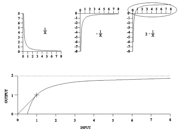
;the result is in the accumulator The derivation of this coding scheme may be of interest to those that wish to better understand its inner workings, and there is more at the end, if you wish to take the plunge! The concept is based on 1/X, which creates a hyperbolic function:
Here, we start with a 1/x function, which generates a hyperbolic graph. We flip the function about the X axis to obtain a -1/X function. Then we add 2 to obtain the third graph, a portion of which is illustrated in magnified form at the bottom. Also, onto this last graph is a straight line from the origin to a point that is tangential to the hyperbola. At this (1,1) point, the function deviates smoothly into a non-linear curve portion, without any discontinuity. The code that creates this is carefully crafted to minimize processor operations. The problem is complicated by the fact that our above graph is only in the first quadrant, dealing with positive inputs and outputs, but the real-world case is to handle bipolar signals. Further, there is the linear portion when the signal is below our threshold (1 in the above graph), and a non-linear one above threshold. In any case, we need to deal with the fact that our real signals do not have the values shown above, that our maximum signals will not exceed +/-1, and therefore our threshold will be much smaller in the final algorithm. The strategy is to obtain a multiplier value (gain) by which to scale the input, which produces an output directly, only needing additional fixed gain to recover the full signal level. Further, if this multiplier value is 1 for all input values that are below our preset threshold, then the linear portion of the resulting function will be produced automatically. We recognize that the transfer function in the non-linear area of the above graph is: Y = 2 - 1/X To properly involve a threshold other than 1, the above expression is: Y = 2 - 12/X ;but, 12 is simply 1... When involving a threshold, we get the following expression: Y = 2t - t2/X ;where t is the threshold selected, and 2t is the saturation limit. If we chose to create a 'gain' value from X, then we need something of the following form: Y/X = 2t/X - t2/X2 ;effectively dividing both sides by X... But we can write this differently: Y/X = 2(t/X) - (t/X)2 Which is convenient, because now we have a t/X term that can be calculated once, and used twice. Realizing that the above function will deliver proper results as a scaling 'gain' value for large values of X, but incorrect values for X that are below our threshold, and also recognizing that the gain value will be 1 if X is equal to t, we finally recognize that t/X for any value of X that is smaller than t will result in a t/X value that is greater than 1, and the FV-1 automatically limits such values to +1. Neat, eh? The only complicated calculation is that of t/X, done with a LOG operation and an EXP operation. The result is stored in an appropriately named register, tovrx. Notice that the algorithm can deal with any threshold, although ones that are 2-n are most convenient. Also, that the correct amount of post gain is required if the threshold is changed. Finally, the offset in the LOG operation must reflect the LOG value of the threshold. As the LOG (LOG2) results in the FV-1 are in 16ths, a threshold of 0.125 (3 bit shift) would require a LOG offset of -3/16. A four bit shift (threshold = 0.0625) would require a LOG offset of -4/16ths. To minimize code, a phase inversion of the gain value is tolerated within the algorithm, which is corrected with a SOF -2,0, but any phase inversion would still be close enough for blues... Now then... We have a means by which to add gain and a clipping function, but this does cause the resulting signal rise and fall times to reflect a much wider output bandwidth than that which came into the block. Since musical frequencies of interest, say, from a guitar, may be safely band limited to perhaps 3KHz, we realize that preceding such a clipping stage with a simple low pass filter will tend to keep the output bandwidth below our Fs/2 limit. Without such filtering, the soft clipper could produce frequencies beyond this Nyquist limit, causing non-harmonic overtones to be folded into our Fs/2 band. For a stage with 12dB of gain (X4), a roll off at 3KHz reduces such aliasing side tones to an imperceptible level. Further, if stages such as these are cascaded to provide extreme sustain, a low pass filter will be needed at the input of each stage. Since the input to a stage is also the output of a preceding stage, let's look at how we can cleverly include a low pass filter at the end of the distortion block. The beauty of this is that the filter can also recover gain, so the final gain producing SOF statements will not be required. When a low pass filter is implemented, there will be feedback around the filter register, and an attenuated input signal added to this feedback value, becoming the next register value. The feedback coefficient and the input attenuation values must sum to 1 for the filter to have unity gain. This means that the filter without the input attenuation would have recursive gain. For a filter using a feedback value of 0.75, the DC gain would be 4. Further yet, such a filter would have a roll off frequency at Fs=32768Hz of about 3.5KHz. This is perfect, as a two operation filter will both filter the signal and provide low frequency gain simultaneously:
These stages can now be cascaded to provide extreme gain and distortion. Notice that the first code statement can be removed if the preceding code is another one of these blocks, because the signal will be in the accumulator and in the previous filter register as well. The last stage however, should not necessarily be filtered, but simply boosted in gain; this provides a wide-band, rich guitar sustain sound. Also, recognize that, with an input of +/-1 maximum, and a threshold of 0.125, the pre-gain maximum signal level will not quite be the ultimate numerical limit of +/-0.25, but will only be +/-0.21875. This means that the filter can tolerate a bit more gain, bringing the output signal closer to the processor's saturation limit. This produces a really fabulous sound. It makes no attempt to duplicate a 'tube' sound, for in many ways the result is an extrapolation of what we like about tubes, but probably not possible with tubes. It is a digitally derived sound that goes beyond tubes, and absolutely in the right direction. Try a cascade of 4 of these... It rips!
Noise Gate / Expander:Finishing a high gain program with an expander can take an otherwise noisy result and make it clean and polished. The FV-1 is especially well adapted to this function, because it can multiply signals by signal-derived numerical values. The code begins with the signal in the accumulator and leaves the gated result in the accumulator. The register 'temp' saves the accumulator value, and is scaled by a value (in this case 0.02) which determines the threshold for gating. This is followed by an absa command that makes sure the result is positive. This absolute signal is then passed into a recursive gain structure that produces a saturation limited signal quickly for large signals and allows a smooth decay when the signal falls below the threshold. When writing the recursive gain signal (gate), a 1.999 coefficient is used to ensure that the final multiply fully passes the input signal during large input signal values (the control signal is fully saturated toward 1.0). The result is very nice and graceful, not at all abrupt or even noticeable; it simply tails off any residual noise!
A quick soft limiting technique was recently brought to my attention by my friend and old time colleague Tony Gambacurta... It uses a cube function to retain the sign of the input signal, and codes really quickly: wrax
temp,-0.33333 This takes a signal in the accumulator and saves it to temp. Simultaneously, the value is flipped in sign and reduced by a factor of 3. Multiplying this by the original temp twice effectively give -(temp^3/3). We then add back the original signal, and it clips to 0.6667 of full scale. Multiplying by 1.5 gives us a full scale signal again. Thanks Tony!
|
||||||||||||||||||||||||||||||||||||||||||||||||||||||||||||||||||||||||||||||||||||||||||||||||||||||||||||||||||||||||||||||||||||||||||||||||||||||||||||||||||||||||||||||||||||||||||||||||||||||||||||||||||||||||||||||||||||||||||||||||||||||||||||||||||||||||||||||||||||||||||||||||||||||||||||||||||